Scaling
In this section, we are not looking at non-linear scalers.
Why Scaling
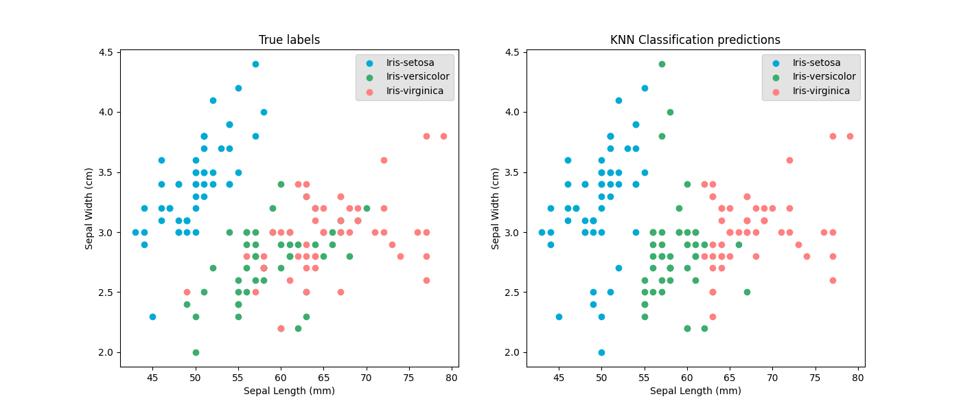
Models base their prediction on the values of the input features. Features can be unfairly treated if they are at different scales.
For example with k nearest neighbours: samples with similar values are predicted to have the same value. So when the values of one feature are much smaller than an the other features, the model will base its almost soiley on just the one small feature.
Scaling input features
Scaling the input features has multiple effects:
- Removing bias towards a feature
- Making the range of values compatible with initiated trainable parameters values
- Increasing the interperability of the trained weights
Scaling targets
Scaling the target is less often necesary because there is often just one target to predict. But it can be useful when the y values is very high due to how the trainable parameters are initialed.
Scaling methods
Normalisation
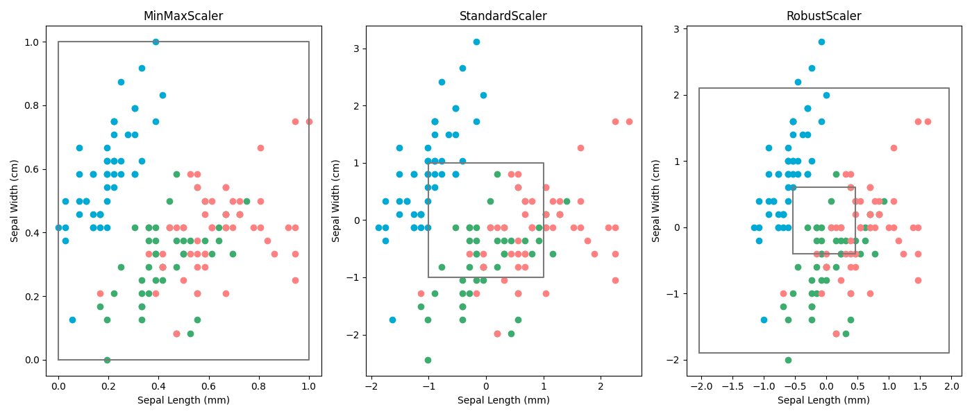
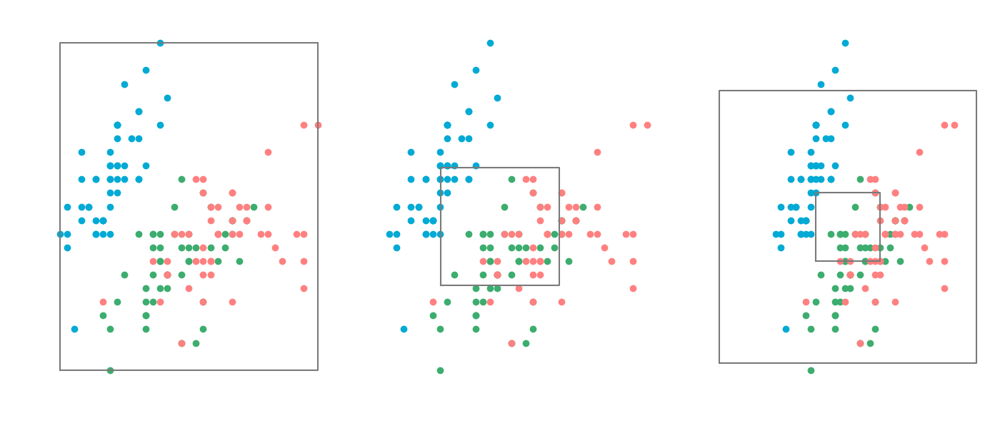
Probably the most straight forward way to scale data is by simply setting the highest value to 1 and the lowest value to 0. And this works quite well to a certain extent. However it's extremely sensitive to outliers, which makes is very unstable.
from sklearn.preprocessing import MinMaxScaler

scaler = MinMaxScaler()

scaler.fit(X_data)
X_data_scaled = scaler.transform(X_data)
# X_data_scaled = scaler.fit_transform(X_data)
Standardisation
Standard deviation
A common way to measure variability in a dataset is by calculating the standard deviation. This statistic tells us how much individual data points deviate from the mean. The formula for standard deviation (SD or ) is:
where:
- is the mean (average) of the data,
- is the number of samples,
- represents each individual data point.
Degrees of freedom
You might notice the in the denominator instead of just . This is not a mistake—it's an important correction.
In statistics, there are two common variations of standard deviation:
- Dividing by (population standard deviation)
- Dividing by (sample standard deviation)
Why do we do this? Well, what we want is the following:
However, the chance that you get samples close to the middle is much larger than the chance of getting more remote samples. This results in a higher likelyhood of having a lower standard deviation estimation when the sample size is small.
To somewhat compensate for the bias to a lower bias, the (Bessel's adjustment) is introduced.
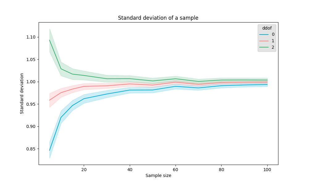

Pandas uses and scipy,
Scikit-learn and
numpy both use (even though the Scipy agrees that is the more correct one but keeping it way for backwards compability reasons).
You can change this by setting ddof=1
A very common way to scale the data is by scaling the values down to the z values. It's a bit more rebust to the biggest and smallest values but still quite sensitive to them due to the quadretic component.
from sklearn.preprocessing import StandardScaler

scaler = StandardScaler()

scaler.fit(X_data)
X_data_scaled = scaler.transform(X_data)
# X_data_scaled = scaler.fit_transform(X_data)
Robust scaling
Quick Ref: Interquartile range
-
Find the 25th percentile (Q1) and the 75th percentile (Q3) of your data.
-
Calculate the IQR:
-
Define the outlier boundaries:
- Lower Bound:
- Upper Bound:
A less common way it to scale using the quantiles, the IQR and the median. However, it's much more stable to outliers then the other two methods.
from sklearn.preprocessing import RobustScaler

scaler = RobustScaler()

scaler.fit(X_data)
X_data_scaled = scaler.transform(X_data)
# X_data_scaled = scaler.fit_transform(X_data)
Other scalers
normalisation and standardisation are by far the most populair once. But, just as we have the robust scaler, there are more: https://scikit-learn.org/stable/auto_examples/preprocessing/plot_all_scaling.html